Introduction to Linear Programing

What is Linear Programming?

Linear programming (LP), also known as linear optimization, is a powerful mathematical method used to find the best possible outcome in a given situation. It’s used to achieve results like maximum profit or minimum cost, where the objective and the constraints are expressed as linear relationships. In essence, LP provides a systematic way to solve optimization problems.

Standard Form

To solve a linear programming problem, we first need to express it in standard form. This is the most common and intuitive way to structure an LP problem and consists of three key components:

A linear objective function to be maximized. This is the quantity you want to optimize. For example: $f(x_{1}, x_{2}) = c_{1}x_{1} + c_{2}x_{2}$
A set of linear inequality constraints. These are the rules or limitations of the problem.

$a_{11}x_{1} + a_{12}x_{2} \leq b_{1} $

$a_{21}x_{1} + a_{22}x_{2} \leq b_{2} $

$ a_{31}x_{1} + a_{32}x_{2} \leq b_{3}$
Non-negative variables. The decision variables must be greater than or equal to zero.

$x_{1} \geq 0 $

$x_{2} \geq 0$

In a more compact matrix notation, the problem can be expressed as:

$\textbf{maximize } \{ \mathbf{c^{T}x} \mid \mathbf{x} \in \mathbb{R}^{n} \land \mathbf{Ax} \leq \mathbf{b} \land \mathbf{x} \geq \mathbf{0} \}$

A Practical Example: The Oil Refinery Problem

Let’s apply these concepts to a real-world scenario. An oil refinery produces two products: jet fuel and gasoline.

The profit is $0.10 per barrel for jet fuel and $0.20 per barrel for gasoline.
The refinery has 10,000 barrels of crude oil available.
A government contract requires at least 1,000 barrels of jet fuel.
A private contract requires at least 2,000 barrels of gasoline.
The truck fleet’s delivery capacity is 180,000 barrel-miles.
Jet fuel is delivered 10 miles away, and gasoline is transported 30 miles away.

The question is: How can the refinery maximize its profit?

Step 1: Formulating the LP Model

First, let’s define our variables. Let $x_1$ be the number of barrels of jet fuel and $x_2$ be the number of barrels of gasoline.

Our objective is to maximize profit, so the objective function is:

$\textbf{Maximize: } P = 0.10x_{1} + 0.20x_{2}$

Next, we establish the constraints based on the problem’s conditions:

$ \begin{aligned} x_{1} + x_{2} &\leq 10000 && \text{(Crude oil availability)} \newline x_{1} &\geq 1000 && \text{(Jet fuel contract)} \newline x_{2} &\geq 2000 && \text{(Gasoline contract)} \newline 10x_{1} + 30x_{2} &\leq 180000 && \text{(Delivery capacity)} \end{aligned} $

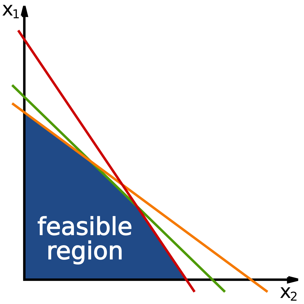
The plot below shows the feasible region—the area where all constraints are satisfied. The optimal solution will lie at one of the vertices of this region.

A graph showing the feasible region for a linear programming problem

Step 2: Converting to Standard Form

The Simplex Method, a common algorithm for solving LP problems, requires a specific format.

First, let’s handle the minimum production requirements. We can introduce new variables, $s_1 = x_1 - 1000$ and $s_2 = x_2 - 2000$, which represent the surplus production above the minimums. This ensures our new variables are non-negative ($s_1, s_2 \geq 0$).

Substituting these into our model gives a new objective function:

$\textbf{Maximize: } P = 0.1(s_1 + 1000) + 0.2(s_2 + 2000) = 0.1s_1 + 0.2s_2 + 500$

And updated constraints:

$ \begin{aligned} (s_1 + 1000) + (s_2 + 2000) &\leq 10000 \implies s_1 + s_2 \leq 7000 \newline 10(s_1 + 1000) + 30(s_2 + 2000) &\leq 180000 \implies 10s_1 + 30s_2 \leq 110000 \newline s_1, s_2 &\geq 0 \end{aligned} $

Next, we convert the inequalities into equalities by introducing slack variables ($k_1, k_2$). These variables represent unused resources.

$ \begin{aligned} s_1 + s_2 + k_1 &= 7000 \newline 10s_1 + 30s_2 + k_2 &= 110000 \end{aligned} $

Our objective function can be rewritten as $Z - 0.1s_1 - 0.2s_2 = 500$.

Step 3: Solving with the Simplex Method

Now we can construct the initial simplex tableau, which is a matrix representation of our system.

Initial Tableau

$s_1$	$s_2$	$k_1$	$k_2$	$Z$	C	Basic Var.	Ratio
1	1	1	0	0	7000	$k_1$	7000/1 = 7000
10	30	0	1	0	110000	$k_2$	110000/30 ≈ 3667 ←
-0.1	-0.2 ↑	0	0	1	500	$Z$

Iteration 1

Identify Pivot Column: Find the most negative entry in the bottom (objective) row. This is -0.2, so the $s_2$ column is our pivot column.
Identify Pivot Row: Calculate the ratio of the constant (C) to the entry in the pivot column for each constraint row. The smallest non-negative ratio determines the pivot row. Here, $110000 / 30 \approx 3667$ is the smallest, making the second row our pivot row.
Pivot: The element at the intersection, 30, is the pivot. We use row operations to make the pivot 1 and all other entries in its column 0.

After performing the row operations, we get the next tableau.

Tableau 2

$s_1$	$s_2$	$k_1$	$k_2$	$Z$	C	Basic Var.	Ratio
2/3	0	1	-1/30	0	10000/3	$k_1$	(10000/3) / (2/3) = 5000 ←
1/3	1	0	1/30	0	11000/3	$s_2$	(11000/3) / (1/3) = 11000
-1/30 ↑	0	0	1/150	1	1233.33	$Z$

Iteration 2 The bottom row still has a negative entry (-1/30), so we repeat the process. The $s_1$ column is the new pivot column. The ratio test identifies the first row as the pivot row.

After pivoting on the 2/3 element, we arrive at the final tableau.

Final Tableau

$s_1$	$s_2$	$k_1$	$k_2$	$Z$	C	Basic Var.
1	0	1.5	-0.05	0	5000	$s_1$
0	1	-0.5	0.05	0	2000	$s_2$
0	0	0.05	0.0033	1	1400	$Z$

Since there are no more negative entries in the bottom row, we have reached the optimal solution.

Step 4: Interpreting the Final Result

From the final tableau, we can read the solution:

$s_1 = 5000$
$s_2 = 2000$
$Z = 1400$

Now, we convert back to our original variables, $x_1$ and $x_2$:

$x_1 = s_1 + 1000 = 5000 + 1000 = 6000$
$x_2 = s_2 + 2000 = 2000 + 2000 = 4000$

The maximum profit is $1400. This is achieved by producing 6,000 barrels of jet fuel and 4,000 barrels of gasoline.

This example is adapted from content available on math.libretexts.org.

Convex Optimization